Translating SPSS to R: One-way Repeated Measures

There’s just no two ways about this: R is just not all that well-configured for repeated measures. Most of the ways of handling repeated measures in R are cumbersome, and some of them just flat-out fail under certain conditions. It’s not a great situation.

Generally speaking, people in the R community do not appear much concerned about this. The argument is usually that mixed linear models is a better way to go because it doesn’t require the same set of restrictive assumptions that repeated measures ANOVA requires. This is fundamentally an argument about sphericity (or, more technically, compound symmetry). If there were no downsides whatsoever to linear mixed models, I’d be OK with this, but it turns out there are some drawbacks that I’ll talk about in some later blog post. Furthermore, repeated measures ANOVA is still far more common in experimental psychology circles, and that’s where I run, so I not only need to be able to do them, I need to be able to teach new graduate students how to do them and how to understand them. R seems designed to make this particularly difficult. In general, R is more difficult to teach with than SPSS, but here’s where it gets particularly ugly.

As usual, I’d like to start with SPSS. However, before I can get into that, I need to spend some time talking about data file formatting. Yes, nuts and bolts stuff gets in there right away. The data come from an experiment (probably fictional—I don’t actually remember where these data came from originally) in which kids were shown the same cartoon on three different days. For those of you who don’t (or didn’t) have small children, kids’ capacity to watch the same thing over and over again and still find it funny is one of the truly amazing feats of childhood. So, the study was done to see if kids would rate the same cartoon less funny after subsequent viewings. Eight kids saw the same cartoon for three consecutive days, and rated how funny it was each time.

So, first we run into the question of “how should the data file be structured?” For between-subjects data, pretty much everybody does it the same way: each line of the data file contains the data for each subject, respectively. This makes sense, since each subject only contributes one observation. But for within-subject data, this isn’t clear. Should it be one observation per line, or one subject per line? It turns out these two ways to do it even have names: one observation per line is called “long” format and one subject per line is called “wide” format.

Wide format looks like this (and is in the file cartoon.xls):

Subj	Day1	Day2	Day3
1	6	5	2
2	5	5	4
3	5	6	3
4	6	5	4
5	7	3	3
6	4	2	1
7	4	4	1
8	5	7	2

So, each line of data has the subject number, and then three observations per subject. Each variable (i.e., “Day2”) represents one measurement on each subject. Here’s what the “long” version of this looks like:

Subj	Trial	Rating
1	Day1	6
2	Day1	5
3	Day1	5
4	Day1	6
5	Day1	7
6	Day1	4
7	Day1	4
8	Day1	5
1	Day2	5
2	Day2	5
3	Day2	6
4	Day2	5
5	Day2	3
6	Day2	2
7	Day2	4
8	Day2	7
1	Day3	2
2	Day3	4
3	Day3	3
4	Day3	4
5	Day3	3
6	Day3	1
7	Day3	1
8	Day3	2

Here, there are 24 lines of data with a variable for subject number (which now has recurring values), a variable representing which day the measurement is, and the rating given.

So, what’s the big deal? Well, it turns out that SPSS (and numerous other stat packages) assume that repeated-measures data is represented in wide format. R can handle both, but there are some advantages to wide-format data even in R, and fortunately it’s pretty easy to go from wide to long in R.

So, the rest of this is going to be done assuming the data are in wide format, as in cartoon.xls.

Basic ANOVA in SPSS
SPSS makes this quite easy. The basic command for this is the GLM command (stands for “general linear model”) and it’s fairly straightforward:

GLM Day1 Day2 Day3
/WSFACTOR Trial 3.

The first line is the command name followed by the list of variables to be included, and the second line defined the repeated measures (or “WS” for “within subjects”) factor, gives that factor a name, and tells SPSS how many levels it has.

It produces rather a lot of output. I’m going to skip the “multivariate tests” output (because if you’re going there, then I’m fully with the “use mixed linear models” argument). The first relevant part of the output is the sphericity diagnostics:

I’m not a big fan of Mauchly’s test because it has low power when sample size is small, but SPSS also produces epsilon estimates so it’s OK. Next is the actual ANOVA table:

It would be nice if it had total SS on it so that it’s easier to compute effect sizes (you can ask SPSS to provide partial eta squared, but that’s not really my preferred measure). Nonetheless, it has pretty much all the other stuff you’d want. There is another piece of output that is provided by default by SPSS, which is contrast output. SPSS assumes, rightly or wrongly, that if you don’t specify what contrasts you want, that you want polynomial contrasts on all your independent variables. Thus, you get this whether you want it or not:

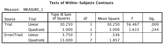
Notice that the error term has only 7 degrees of freedom, and that each contrast has its own error term. This is a particular choice on the part of the SPSS developers. What this means is that the error terms are unique and thus do not require the sphericity assumption. It also means that these tests exactly match what you get if you do your repeated measures contrasts by t-test (more on that in a bit).

Some people prefer pooling the error term, that is, using the error term from the original RM ANOVA (the one with 14 df), but that requires the sphericity assumption, and the test doesn’t match the contrast t-test. This is the kind of thing reasonable people can disagree about (again, I’m not in the business of telling people how to adjudicate arguments like that on this blog—for now). It would be nice if SPSS gave the option to include the tests computed that way. Note that technically you can compute it yourself by hand if you want to, but you have to make sure you normalize the contrast vectors to make this work.

Basic ANOVA in R, Wide Format
R is not in the business of making this easy. Essentially, the way you do this in R is to set up a linear model with the “lm()” function, and then tell SPSS that’s it’s really a repeated measures ANOVA using the “Anova()” command out of the “car” package. It’s a little more laborious, but for a one-way it’s not really that bad. Again, assuming the data has been read in and attached, the code looks something like this (with annotations in the code this time):

## load “car” to get the Anova() function
library(car)

## Create a model of the within-subjects factors
Anv1 = lm(cbind(Day1, Day2, Day3)~1)

## Create a labeled factor for w-s factors
Trial = factor(c("Day1", "Day2", "Day3"))

## do the ANOVA. “idata” and “idesign” tell Anova() how to
## structure within-subjects factors
Anv2 = Anova(Anv1, idata=data.frame(Trial), idesign=~Trial)

## Get out the ANOVA tables and adjustments
summary(Anv2, multivariate=F)

Somewhat more than SPSS indeed. Here’s the output:

Univariate Type III Repeated-Measures ANOVA Assuming Sphericity

                SS num Df Error SS den Df       F    Pr(>F)    
(Intercept) 408.37      1   18.625      7 153.483 5.132e-06 ***
Trial        33.25      2   16.750     14  13.896 0.0004735 ***
---
Signif. codes:  0 ‘***’ 0.001 ‘**’ 0.01 ‘*’ 0.05 ‘.’ 0.1 ‘ ’ 1


Mauchly Tests for Sphericity

      Test statistic p-value
Trial        0.66533 0.29452


Greenhouse-Geisser and Huynh-Feldt Corrections
 for Departure from Sphericity

       GG eps Pr(>F[GG])   
Trial 0.74925   0.001856 **
---
Signif. codes:  0 ‘***’ 0.001 ‘**’ 0.01 ‘*’ 0.05 ‘.’ 0.1 ‘ ’ 1

         HF eps   Pr(>F[HF])
Trial 0.9077505 0.0007808673

Unlike SPSS, no contrasts are provided by default, but all the relevant output matches. Unlike with SPSS, R doesn’t compute what the adjusted degrees of freedom are, so you have to compute those by hand. Not hard, but slightly annoying—isn’t computing stuff kind of the point of doing it in software in the first place? But I digress.

So, the basic ANOVA is not too bad to do in R with wide-format data. Let’s take a look at contrasts in both packages.

Custom Contrasts in SPSS
There are two relatively straightforward ways to do custom contrasts in SPSS: as t-tests and as part of the GLM. First, the contrasts. By default it provides polynomials so let’s do something else. Let’s try two: (-2 1 1) to compare the first viewing with the mean of the later viewings (that is, is it only funny once?), and then (0 1 -1) to compare the second and third viewings. To do those as t-test in SPSS, we just compute the relevant variables and test whether or not those equal zero:

COMPUTE Day1vs23 = -2*Day1 + Day2 + Day3.
COMPUTE Day2vs3 = Day2 - Day3.
EXECUTE.

T-TEST
/VAR Day1vs23 Day2vs3 /TESTVAL 0.

Why on earth SPSS requires the EXECUTE statement is beyond me, but I’ve complained about that before so I’ll leave it alone for now. Here’s the output:

Apparently, even for the kids, the cartoon is getting less funny over repeated viewings; even the second and third viewing are different. Anyway, that gets the job done. It is also possible, however, to do the contrasts right within the GLM itself. To do that, you need to tell SPSS to run contrasts in the WSFACTOR subcommand. It looks like this:

GLM Day1 TO Day3
/WSFACTOR Trial 3 SPECIAL(1 1 1
-2 1 1
0 1 -1).

You see the “-2 1 1” vector and the “0 1 -1” vectors there in the command. Why the “1 1 1” vector is required is a mystery to me, since you’re not allowed to put anything else in there. Bizarre. Anyway, the first part of the output is the same as the previous GLM command, but the contrast output is different:

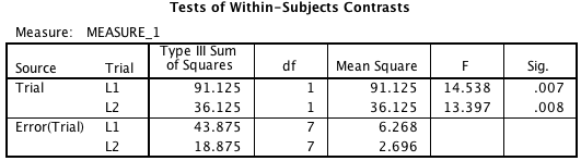
Note the p-values are the same as the previous output, and those Fs are the square of the ts from the previous output. SPSS will also supply the partial eta squared values for the contrasts if you ask it to with at “/PRINT ETASQ” command. Again, not my preferred measure of effect size.

Custom Contrasts in R, Wide Format
The “Anova()” procedure in R doesn’t support contrasts at all, so you more or less have to do it by t-test. The good news is that R understands matrix multiplication, so you can at least make the code short. First, the SPSS way, writing out the contrast coefficients implicitly:

Day1vs23 = -2*Day1 + Day2 + Day3
t.test(Day1vs23)
Day2vs3 = Day2 - Day3
t.test(Day2vs3)

There is a slightly quicker way to do this that relies on R’s ability to do matrix multiplication. I prefer this because it lets you write out the contrast vectors explicitly:

Day1vs23 = cbind(Day1, Day2, Day3) %*% c(-2, 1, 1)
t.test(Day1vs23)
Day2vs3 = cbind(Day1, Day2, Day3) %*% c(0, 1, -1)
t.test(Day1vs23)

And here are the results (they’re identical for both code snippets above):

One Sample t-test

data: Day1vs23
t = -3.8129, df = 7, p-value = 0.006603
alternative hypothesis: true mean is not equal to 0
95 percent confidence interval:
-5.468036 -1.281964
sample estimates:
mean of x
-3.375

One Sample t-test

data: Day2vs3
t = 3.6602, df = 7, p-value = 0.008068
alternative hypothesis: true mean is not equal to 0
95 percent confidence interval:
0.7521863 3.4978137
sample estimates:
mean of x
2.125

So, as it should, R agrees with SPSS on these tests. All is well in the universe, right? Well, maybe, unless (a) you have long-format data, or (b) you’d like to use pooled error terms in your contrast tests. In the case of (b), those tests will not necessarily agree with SPSS, though of course SPSS will let you compute those tests if you really want them, as all the appropriate information is on the printout. So, let’s take a look at R with long-format data.

Conversion to Long Format in R
The good news is that if you want long-format data in R and you have wide-format data, it’s pretty easy to transform the data. (This is also possible in SPSS, but it’s moderately cumbersome to do it and I have to look it up every time.) Let’s say the data is in a data frame called “cartoon.” I’m going to put it into long format with a command called “melt()” from the “reshape2” library. The commands look like this:

detach(cartoon)
library(reshape2)
cartoon.lng = melt(cartoon, id.vars="Subj", variable.name="Trial", value.name="Rating")

Note that the “detach()” isn’t technically necessary. This produces a data frame called “cartoon.lng” that looks exactly like the long-format table earlier in the post.

Basic ANOVA in R, Long Format
R offers multiple ways to handle the ANOVA in wide format. The simplest way is to use the “ezANOVA()” function out of the “ez” package. Essentially this is really just a wrapper for the “car::Anova()” function we used last time, but it makes things slightly easier, particularly for more complex designs. For this one-way design, the simplicity gain isn’t that large. The code looks like this:

library(ez)
cartoon.lng$SubjF = factor(cartoon.lng$Subj)
ezANOVA(cartoon.lng, dv = Rating, wid = SubjF, within = Trial, detailed=T)

So, that code loads the “ez” library, creates a new variable in the “cartoon.lng” data frame that is the “Subj” variable represented as a factor, then does the ANOVA with “Rating” as the dependent variable (hence “dv”), notes that the variable that identifies subject (the “wid”) is the variable “SubjF” and the within-subjects variable (“within”) is “Trial”. Here’s the output:

$ANOVA
       Effect DFn DFd     SSn    SSd         F            p p<.05       ges
1 (Intercept)   1   7 408.375 18.625 153.48322 5.131880e-06     * 0.9202817
2       Trial   2  14  33.250 16.750  13.89552 4.734931e-04     * 0.4845173

$`Mauchly's Test for Sphericity`
  Effect         W         p p<.05
2  Trial 0.6653301 0.2945177      

$`Sphericity Corrections`
  Effect       GGe      p[GG] p[GG]<.05       HFe        p[HF] p[HF]<.05
2  Trial 0.7492489 0.00185552         * 0.9077505 0.0007808673         *

And of course the output matches the wide-format use of “car::Anova()” since it’s actually using that procedure to do the actual ANOVA. Note that this automatically provides an estimate of effect size; that’s the “ges” on the printout. This is the “generalized eta squared” measure from Bakeman (2005), which is not really a standard in Psychology but is a defensible choice and is certainly not unheard-of.

The minor down side to ezANOVA is that it doesn’t let you do contrasts. Well, actually, you can, but to do so you need to have ezANOVA return the lm object, which it will do, but to understand how to use that you need to do what’s in the next section anyway, so I’ll go through that.

Custom Contrasts in R, Wide Format
This is where I dislike doing things in the long format in R, because the only straightforward way to do the contrasts provides you with what you have to do by hand in SPSS, that is, pooled error terms.

First, it is actually possible to do the ANOVA with long-format data without using “ezANOVA().” However, if you do it this way, you do not get sphericity diagnostics, which seems like a really bad idea to me. (Look, I get that the logic is that mixed linear models don’t make this assumption, but how do you know how important that assumption is if you don’t get information about it? Seems backward to me.) Anyway, you do this in R by specifying the within-subjects error term in the specification of the model. It looks like this:

Anv = aov(Rating ~ Trial + Error(SubjF/Trial), data=cartoon.lng)
summary(Anv)

That whole “Error(SubjF/Trial)” is the specification of the within-subjects error term. Here’s the output:

Error: SubjF
          Df Sum Sq Mean Sq F value Pr(>F)
Residuals  7  18.62   2.661               

Error: SubjF:Trial
          Df Sum Sq Mean Sq F value   Pr(>F)    
Trial      2  33.25  16.625    13.9 0.000473 ***
Residuals 14  16.75   1.196                     
---
Signif. codes:  0 ‘***’ 0.001 ‘**’ 0.01 ‘*’ 0.05 ‘.’ 0.1 ‘ ’ 1

How can you not love that? The p-value to six decimal places, but the F-value to only two. Really? (Question for anyone who happens to read this from the R community: are there journals out there that request six decimal places for the p-value? If so, how many decimal places do they want for the F? Because in psychology the convention is for two decimal places in the F-value and no more than 3 for the p-value.) And while the relevant stuff matches the other SPSS and R outputs, as I noted, there’s no Mauchly test or sphericity epsilons there.

So that’s not great, but what about contrasts? Well, you do it pretty much how you do contrasts in between-subjects ANOVA in R: you set up the contrast, run the ANOVA, and you ask R to split up the output in the summary. It looks like this:

contrasts(cartoon.lng$Trial) = cbind(c(-2, 1, 1), c(0, 1, -1))
Anv = aov(Rating ~ Trial + Error(SubjF/Trial), data=cartoon.lng)
summary(Anv, split=list(Trial=list("Day1vs23"=1, "Day2vs3"=2)))

I know, pretty, isn’t it? Here’s the output:

Error: SubjF
          Df Sum Sq Mean Sq F value Pr(>F)
Residuals  7  18.62   2.661               

Error: SubjF:Trial
                  Df Sum Sq Mean Sq F value   Pr(>F)    
Trial              2  33.25  16.625   13.90 0.000473 ***
  Trial: Day1vs23  1  15.19  15.188   12.69 0.003120 ** 
  Trial: Day2vs3   1  18.06  18.062   15.10 0.001648 ** 
Residuals         14  16.75   1.196                     
---
Signif. codes:  0 ‘***’ 0.001 ‘**’ 0.01 ‘*’ 0.05 ‘.’ 0.1 ‘ ’ 1

So, there, contrasts in long-format repeated-measures ANOVA. You’ll note that these results do not agree with the results generated by SPSS or by the t-tests we did on the wide-format data. As I mentioned before, these use the pooled error term, which means you have to be especially careful with sphericity here.

Note that you can get the same results from SPSS with a little hand computation. If you go back to the “L1” line in the SPSS output when we did this contrast, note that the SS for the contrast was 91.125. The squared length of the (-2 1 1) vector is six, so if we take that SS and divide by six, we get 15.188, which is the SS for the contrast in the wide format for R, so we could compute the same 12.69 F-value by dividing by the (pooled) MSE of 1.196. So this method is available to SPSS users, though it’s kind of a hassle since you have to do a lot of the computations by hand.

Frankly, I’m not a fan of doing contrasts this way, which means if I’m using R, I pretty much have to stick to wide-format data. That’s basically OK in this context, but it can get a little cumbersome for ANOVAs with many within-subjects factors. That’ll be the subject for the next post…